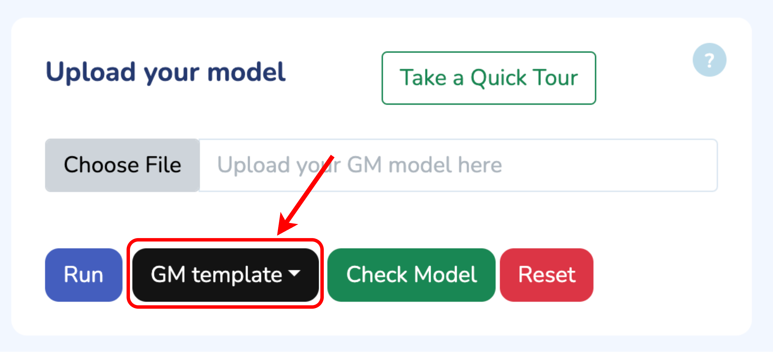
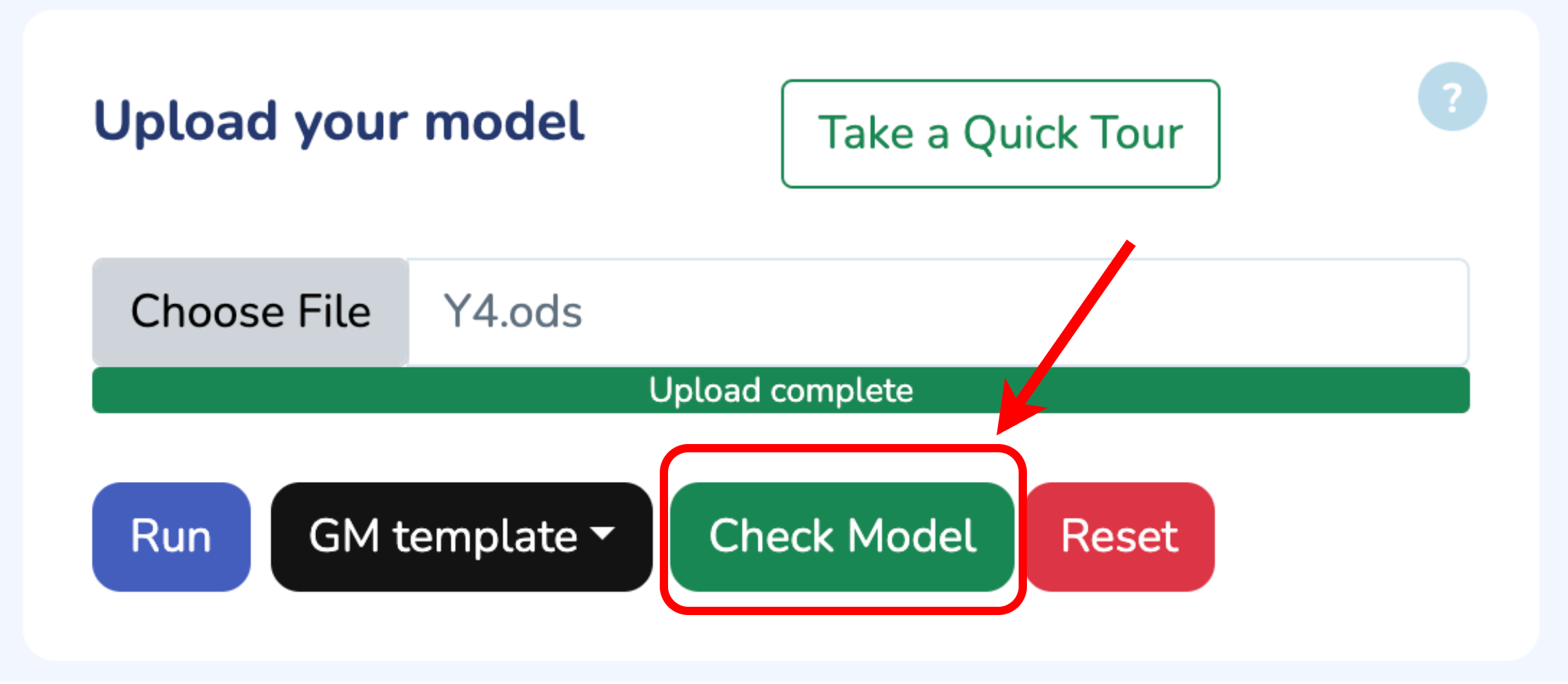
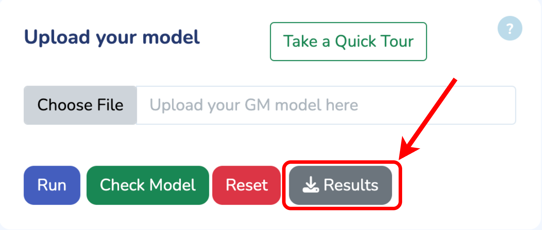
To begin, upload your Growth Mechanics (.ods) model by clicking “Choose File.” If you need the template, click “Download GM Template.” Once uploaded, verify your model by clicking “Check Model.” Any errors will be flagged immediately. When you’re all set, click “Run” to start optimizing your model.
Upload your model

Number of Time Points
Maximum Growth rate
h-1
Average of Total Protein Concentration
[g L-1]
Total Simulation Time
h
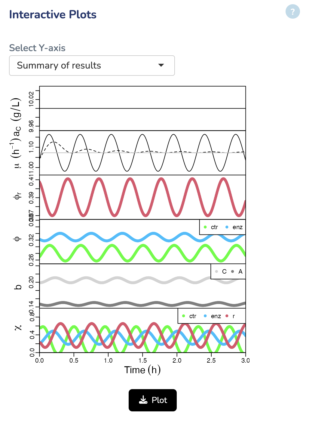
Interactive Plots
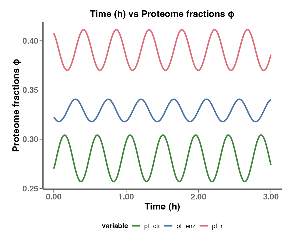
In this section, you can visualize the results by selecting different axes, such as Growth Rate, Protein Fractions/Concentrations, Fluxes, and more.
Your Growth Mechanics Model
Here, you can view your uploaded GM model. The first tab displays the Mass Fraction matrix (M) of your model. Even after optimization, you can modify any parameters and rerun the optimization by clicking "Run" in the last tab to see the changes. Additionally, you can download the updated model by clicking "Download" in the "rho" tab.
Here, you can view your uploaded GM model. The first tab displays the Mass Fraction matrix (M) of your model. Even after optimization, you can modify any parameters and rerun the optimization by clicking "Run" in the last tab to see the changes. Additionally, you can download the updated model by clicking "Download" in the "rho" tab.
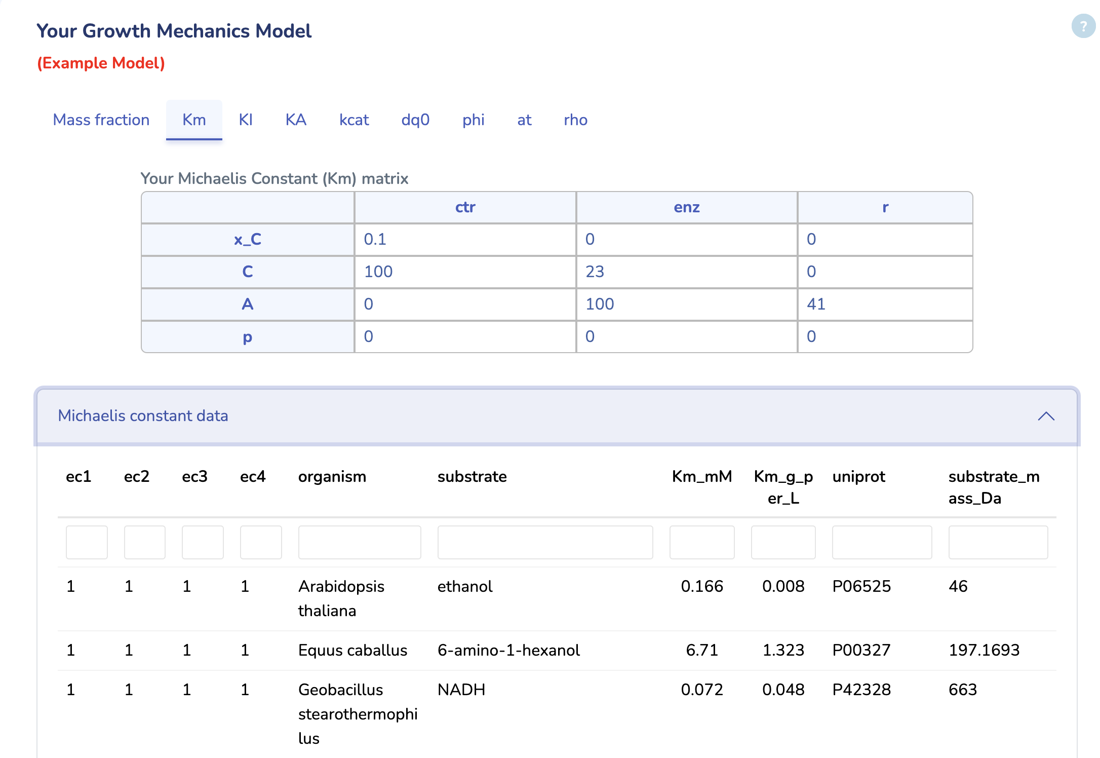
This section displays the Michaelis Constant (Km) matrix of your uploaded GM model. Make sure each substrate in your reactions has a valid Km value; otherwise, a default value of 0.1 g/L will be used. You can also search for Km values in the table below, sourced from the BRENDA database. Please ensure Km values are mass balanced and converted to g/L by multiplying the Km values in molar units by the molecular weights of the respective substrates.
This section displays the Inhibition Constant (KI) matrix of your uploaded GM model. You can modify the values directly here.
This section displays the Activation constant (KA) matrix of your uploaded GM model. You can modify the values directly here.
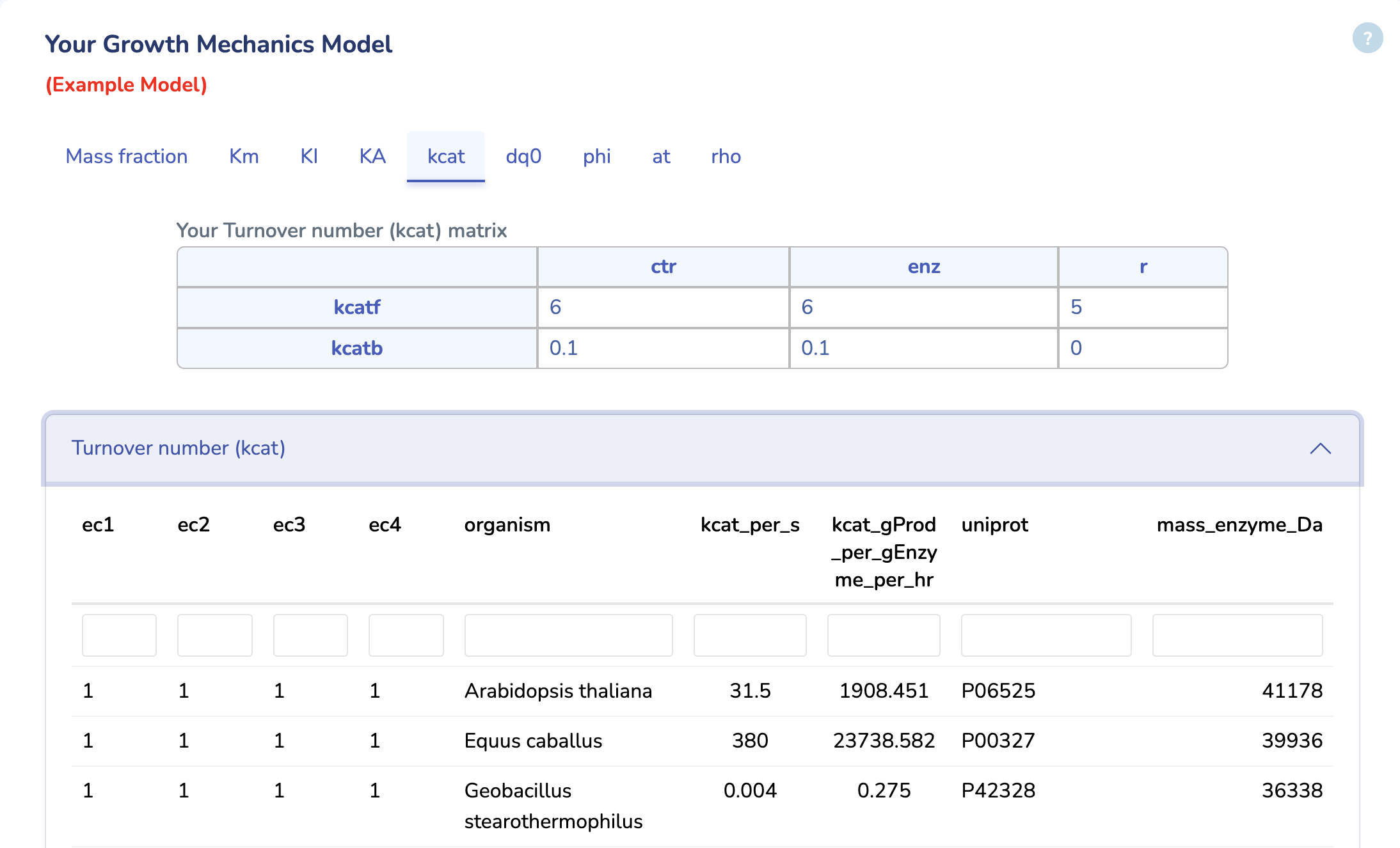
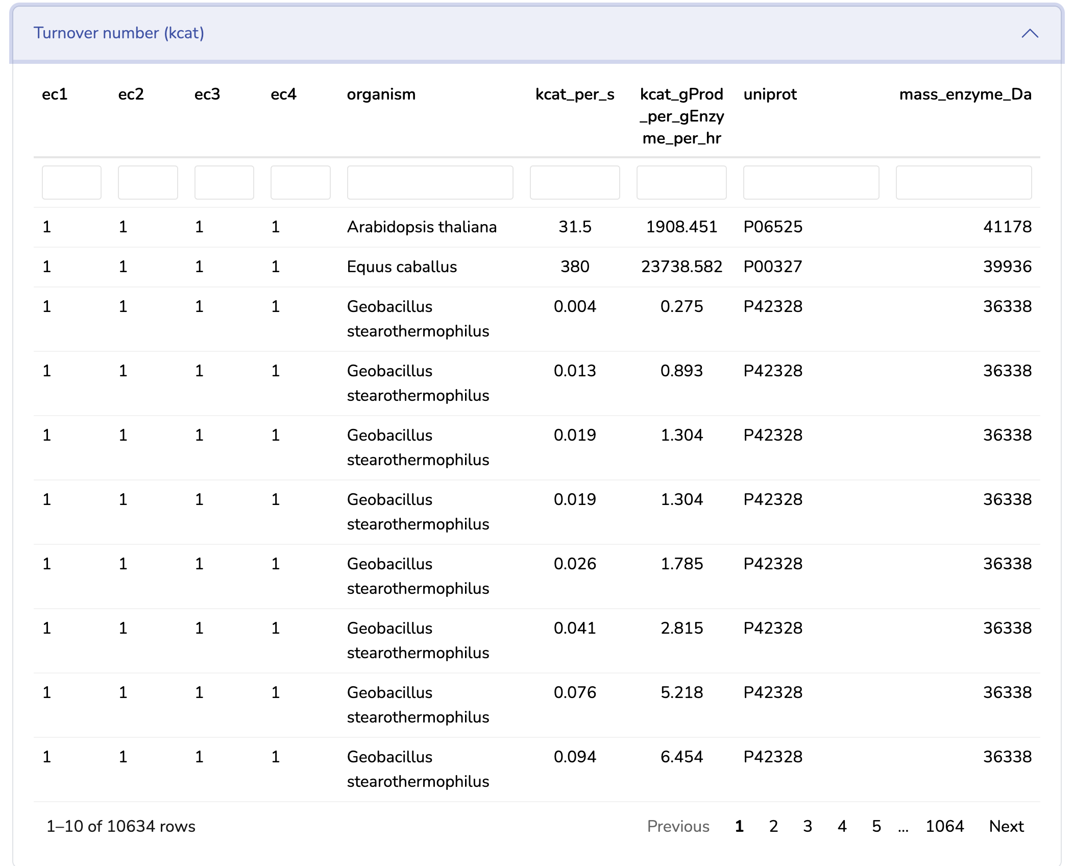
This section displays the Turnover Number (kcat) matrix of your uploaded GM model. You can search for kcat values in the table below, sourced from the BRENDA database. Ensure that kcat values are mass balanced and converted to 1/h (mass of product/mass of enzyme/hour) by multiplying the kcat values in 1/h units by the molecular weight of the respective product and dividing by the mass of its enzyme. "kcatf" and "kcatb" indicates the kcat for forward and backward reactions, respectively.
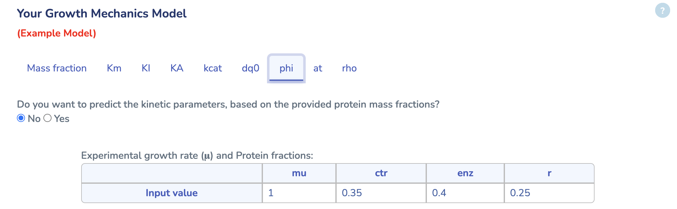
In this section you can enter experimental values for the growth rate (μ) and protein mass fractions (ϕ) for each reaction. Select “Yes” if you’d like the app to estimate your kinetic parameters from these inputs automatically.
This section displays the Oscillation Amplitude (dq₀) matrix for your uploaded Growth Mechanics model. You can edit the values here to set the initial perturbations in growth‐rate coordinates for simulating metabolic oscillations.
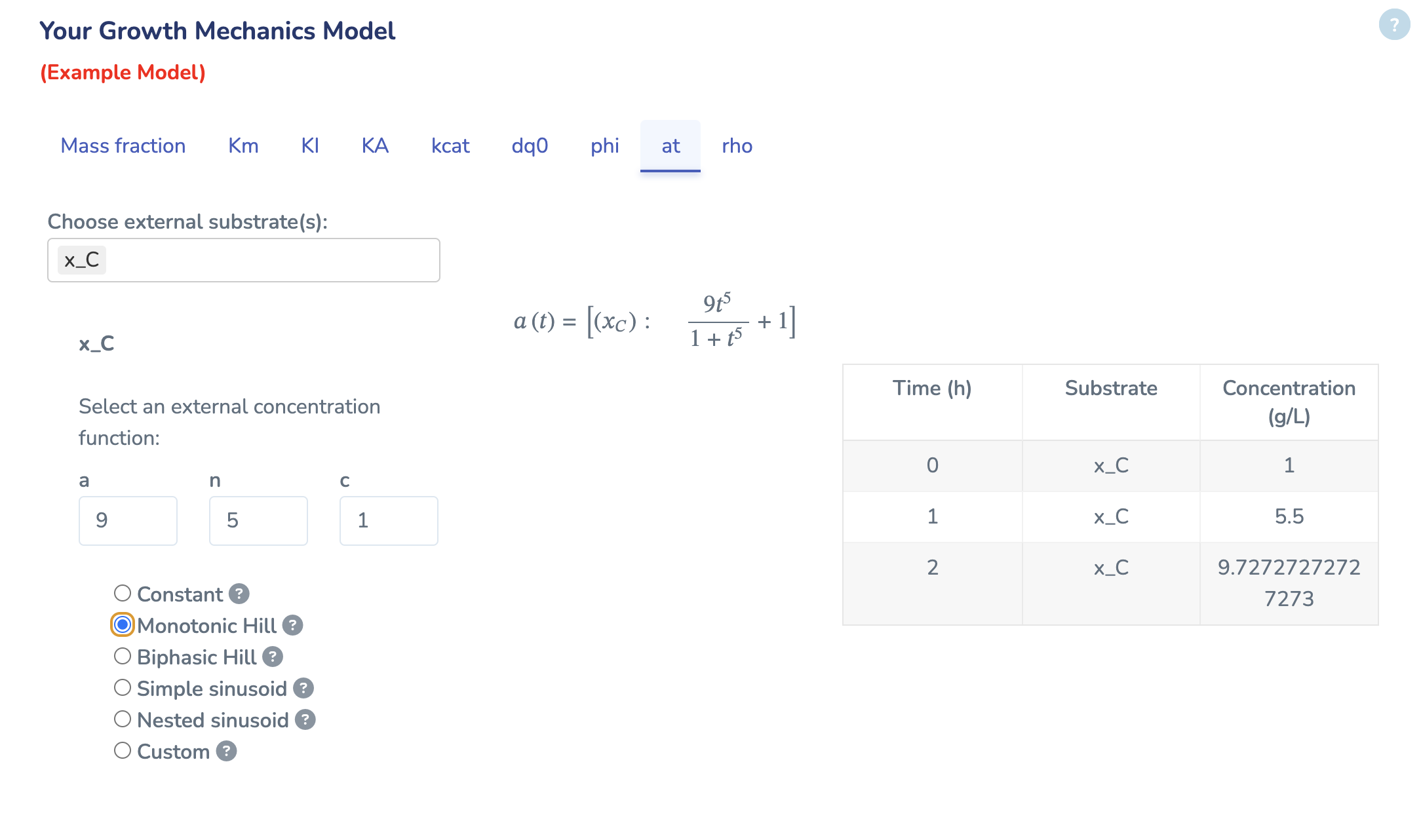
Here you define time‐varying external concentrations for each transporter. Select one of the built‐in function - Constant, Monotonic Hill, Biphasic Hill, Simple Sinusoid, Nested Sinusoid - or choose “Custom” to enter your own R expression. For each transporter, pick its function and adjust the parameter fields as needed. By selecting the function, you will see how the concentrations evolve over the first three hours in the example table below.
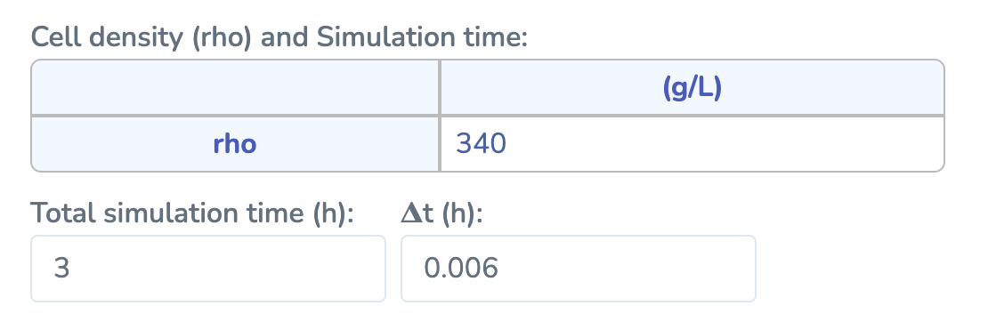
In this section, enter the cell density (ρ) for your model as a single numeric value greater than zero. Specify Total Simulation Time (must be < 30 hours) and Time Step ΔT (must be < 1 hour) to control the duration and resolution of your simulation. After updating these values, click “Run” to start the numerical simulation.
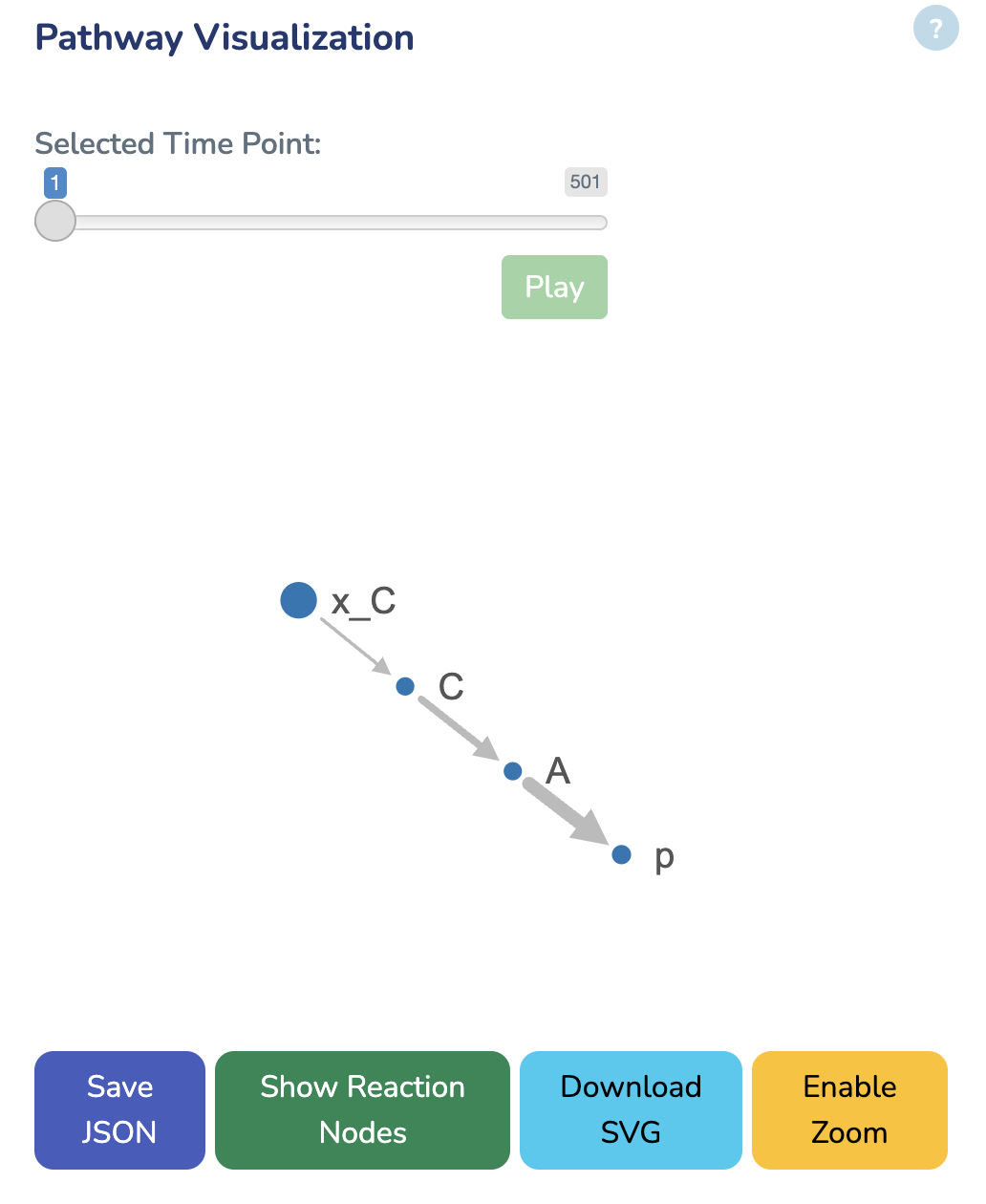
Pathway Visualization
In this section, you can explore the network visualization of your Growth Mechanics model. Dot size reflects metabolite concentrations. Line thickness reflects protein concentrations. Click the Play button or move the slider to animate the network over time - concentrations and fluxes will update at each time point. Use the download link below to save the current visualization.